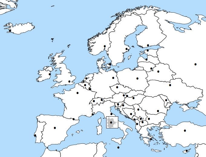
Imagine you want to travel around Europe. You want to see the sights, and visit as many European capital cities as possible, but you’re on a budget; flights can get expensive, so you plan to travel by rail and bus. To make your funds stretch as far as possible, you need to plan a route that will take you to all of the cities on your list for the cheapest price, before heading home again.

This is known as the Travelling Salesman Problem, and it’s a classic puzzle in computer science, operations research, and graph theory. While the problem itself may seem fairly straightforward, finding a solution proves deceptively challenging. Worse still, if you’ve found a solution that you think is the best, there is no quick or easy way to verify that it is in fact the optimal route.

What Makes It So Challenging?

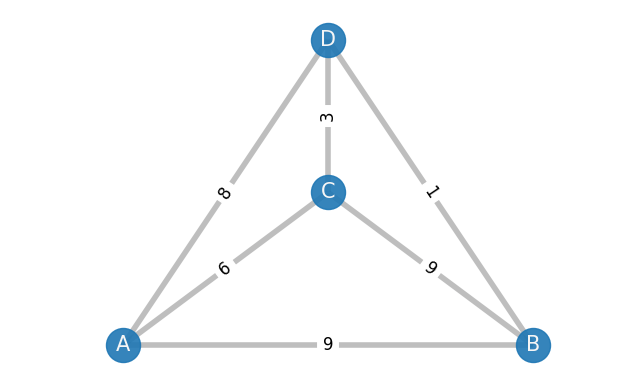
Let’s model the problem with a graph. We’ll use nodes to represent the cities, and add an edge wherever we have a transport link between cities. The numbers on the edges represent the cost of the journey.

This graph is known as a complete graph, since every node is directly connected to every other one by an edge.

Let’s say you live in city A. You have 6 choices as to the order in which you can visit the other cities (starting and finishing at A):

ABCDA, ABDCA, ACBDA, ACDBA, ADBCA, ADCBA

Let’s also assume, for the sake of simplicity, that the cost of the journey from A to B is the same as the cost from B to A, so it doesn’t matter which direction you travel in. This means that the tour: ABCDA is actually the same as ADCBA, just traversed in the opposite direction. This cuts the number of possible routes in half, leaving us with 3 to consider:

ABCDA, ABDCA, ACBDA

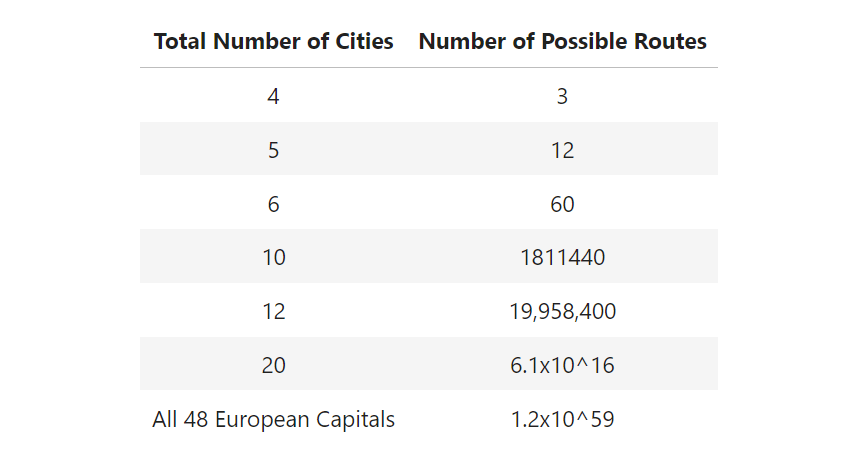
Well that’s not so complicated to solve, right? We could just check each of the possibilities in turn and see which one is the cheapest. And you’d be right: to actually solve the problem (and guarantee you’ve found the best route) this is the only way it can be done. However, when we start looking at larger graphs, the number of possibilities increases dramatically:

As you can see, the problem gets out of hand pretty quickly, making it very difficult, if not impossible, to find a solution. To give these numbers some context, with just 20 cities, we’re looking at a number of routes comparable to the number of grains of sand on Earth! If we relax the constraint that the journeys cost the same in both directions, we would need to double the number of possible routes, making it even more challenging to solve.

Heuristic Methods

As we’ve seen so far, there is no definitive solution to this problem (except a brute force approach). However, there are some heuristic methods we can use to give us an approximate solution. While the result may not be optimal, these algorithms give us answers that are sufficient for many practical use cases, and can be computed in a much more reasonable time scale.

Nearest Neighbour Algorithm

The Nearest Neighbour algorithm is one of the simplest approaches to finding a solution. We begin at the start node, A, and then visit the lowest cost adjacent node. From this new node, we repeat, finding the cheapest node to visit that we have not already been to. Once all nodes have been visited, we then return to the start.

For the above graph, the algorithm would look something like this:

• Start at A
• The cheapest unvisited adjacent node is C (cost=6)
• From C, the cheapest unvisited adjacent node is D (cost=3)
• From D, the only remaining unvisited node is B (cost=1)
• From B, we return to the start node, A (cost=9)

This gives us the route A-C-D-B-A with a total cost of 19. In this case, this is the best solution we can find.

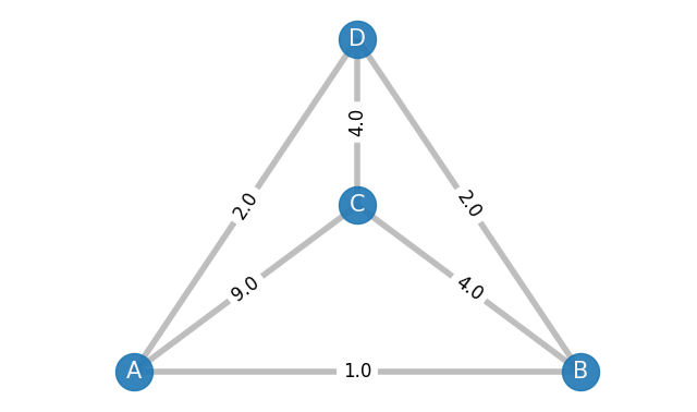
However, this algorithm doesn’t always give us the best solution:

Applying the same steps to this graph gives us the route A-B-D-C-A which has a total cost of 16 (=1+2+4+9). But this is not the optimal route: the path A-B-C-D-A has a total cost of 11 (=1+4+4+2).

Greedy Algorithm:

A ‘Greedy Algorithm’ is one that makes the best choice at each step, it does not consider how its choices impact the solution as a whole, so long as the immediate choice looks like it is heading in the right direction. The Nearest Neighbour approach is also an example of a greedy algorithm.

Another way we could find a solution is to sort all of our edges by their cost, lowest to highest. We can repeatedly add the shortest edges to our solution, ensuring that they satisfy some constraints:

• adding an edge does not form a cycle- unless this cycle visits every node (so if there are 4 nodes, we don’t want a cycle that includes 3 nodes)
• adding an edge does not result in a node with more than 2 edges connecting to it

These constraints will ensure that we only visit each node exactly once before returning to the start. Let’s apply this method to the first example again.

• The lowest cost edge in this graph is DB (cost=1). We add this to our solution
• The next lowest cost edge is DC (cost=3). We add this to our solution
• The next lowest cost edge is AC (cost=6). We add this to our solution
• The next lowest cost edge is AD (cost=8), but we already have 2 edges that connect to D (DB and DC), so we ignore this edge
• If we have edges of equal weight that satisfy all constraints, it does not matter which one we pick. In this case AB and BC both cost 9, however adding BC would violate both constraints: There would be 3 edges in our solution that connect C. It would also create a cycle, CBD, which does not include all nodes. Therefore, we must choose the edge AB (cost=9)
• We now have all 4 edges: DB, DC, AC, AB. Notice that each letter appears exactly twice in this list. We can construct a tour out of these edges that starts and ends at A: ABDCA this will have cost (19). This is the same solution found by the Nearest Neighbour method. Again, in this case, we have found an optimal solution.

Genetic Algorithm

A Genetic Algorithm is a machine learning technique modelled on biological evolution. We start with a random sequence, visiting the cities in a completely random order, and repeatedly improve upon this route until we find ‘good enough’ solution. Again, this solution may or may not be optimal.

For more information about Genetic Algorithms, check out this article

Real-world Uses

The Travelling Salesman Problem has many real-world applications. As you might guess, it can be used for delivery and distribution systems in order to optimise routes and improve warehouse operations. However, it also crops up in the manufacture of circuit boards and X-ray crystallography (the analysis of the structure of crystals).

The problem is deceptively simple, and it is not known whether there exists an efficient solution, but one has not yet been found. It is also a great example of a time-accuracy trade off, where achieving an optimal solution is unrealistic, whereas a faster, though less accurate solution, is often more practical. This is a common theme in many areas of problem solving and decision making.

Whether planning a trip across Europe or optimizing delivery routes, understanding the Travelling Salesman Problem and its solutions can save time, and money. Ultimately, it highlights the importance of finding effective and efficient solutions in a world where the right answer is not always available.

---