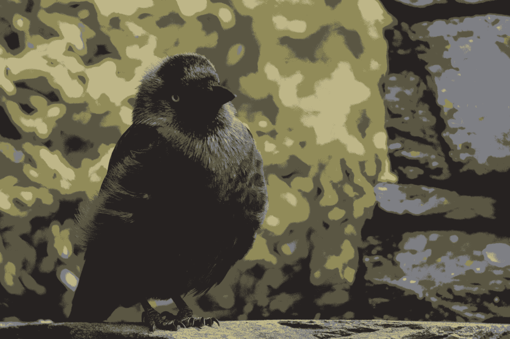
LEFT: Original Photograph, RIGHT: Segmented image (5 colours/segments)

Looking at the images above, we see an example of an image posterization filter that gives images a cartoon-like appearance, but behind the scenes, this filter is actually using a machine learning algorithm known as clustering.

Before exploring into how this process works and seeing how we can implement it in Python, let’s take a look at why we might want to do this in the first place.

Image Segmentation

In a normal photograph, a pixel can take one of roughly 16.7 million different colours. In this processed image, however, there are only 5 different colours. We’ve split all of the pixels into 5 different groups, segmenting the image into these different colour-regions.

We’ve also cut down on the amount of noise and variation within the image. So, if this were to be used in some other machine learning application, we’ve just massively reduced the amount of data that needs to be processed, especially if this were applied to a whole library of images.

Even though we’ve simplified this image, we’ve still retained most of the important structural data. We are still able to identify shapes and forms, shadows and highlights, and many different textures and patterns. All the information that tells us that this is a picture of a bird sat on a wall, is still there.

This process doesn’t just apply to images either. We can use the same tools on a variety of different datasets in other contexts, to simplify them and reduce the amount of data processing required.

Beyond just reducing data processing requirements, this algorithm has more direct applications too, as it allows us to more easily identify features within an image. For example, the lake on the left side of the image below is almost entirely one pixel colour, and distinct from all of the pixels around the lake, making it easy to isolate.

This technique could, for example, be used to track the size of polar ice-caps; by taking an image, applying this filter to identify ice and ocean pixels, you can then easily work out the area covered by ice.

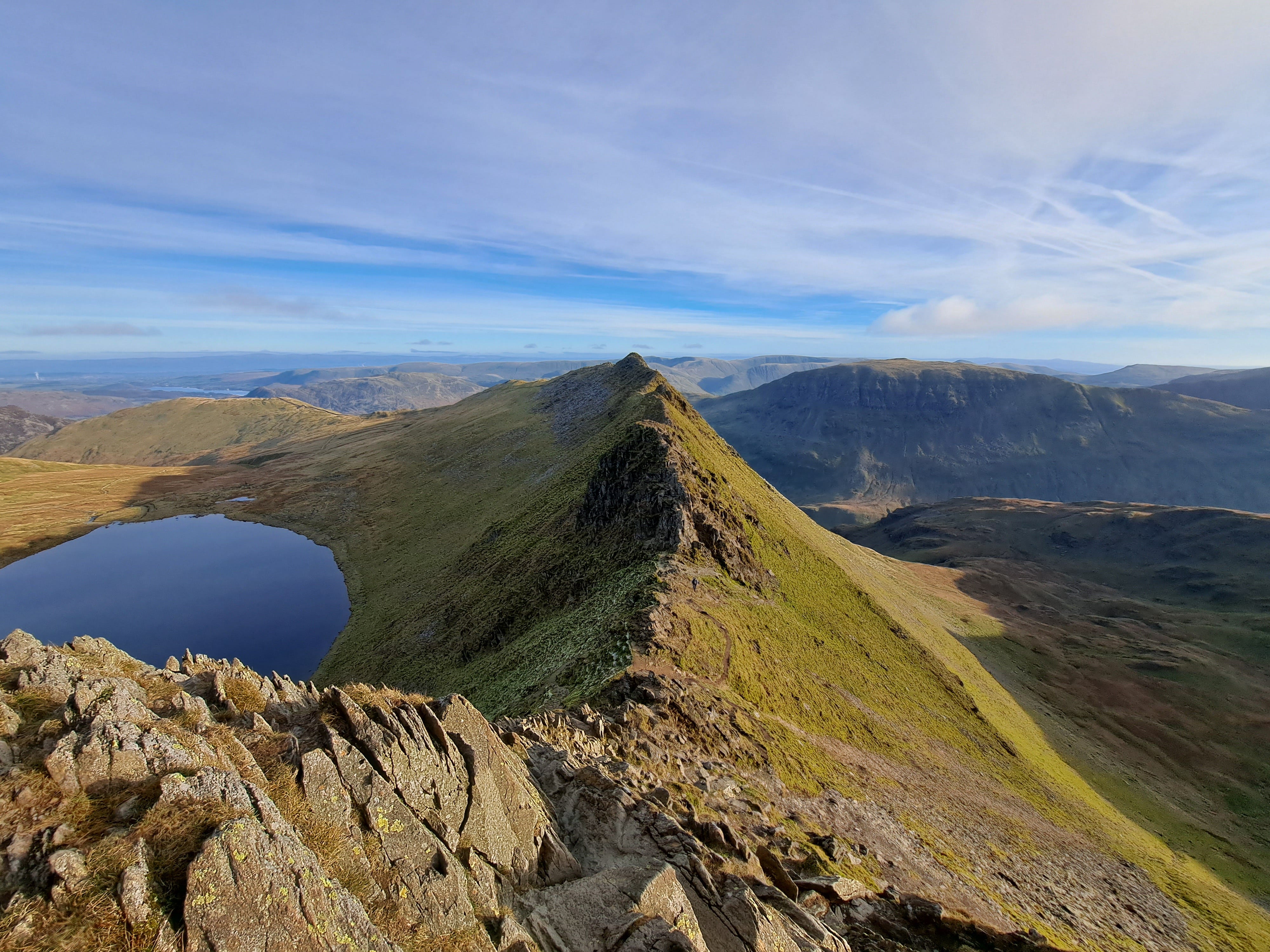
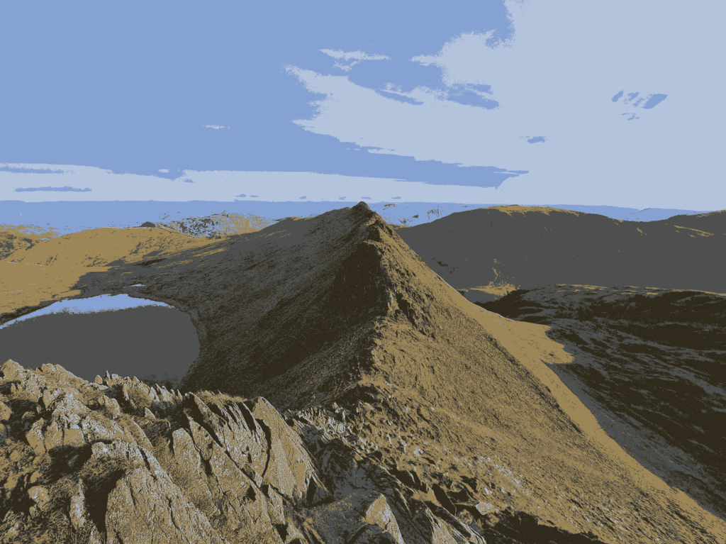
LEFT: original photograph, RIGHT: segmented image (5 colours)

Clustering

The machine learning technique powering this process is known as clustering. It’s a process used to identify clusters, or groups, within a dataset. For example, with an image, we identify groups of pixels that are a similar colour. The number of groups we wish to find is one of the parameters of the algorithm.

There are 3 main different types of clustering: density based, centroid based, and hierarchical, each of which has many different algorithms that can be used depending on the situation. For this article, we will be implementing a centroid-based algorithm known as K-Means clustering.

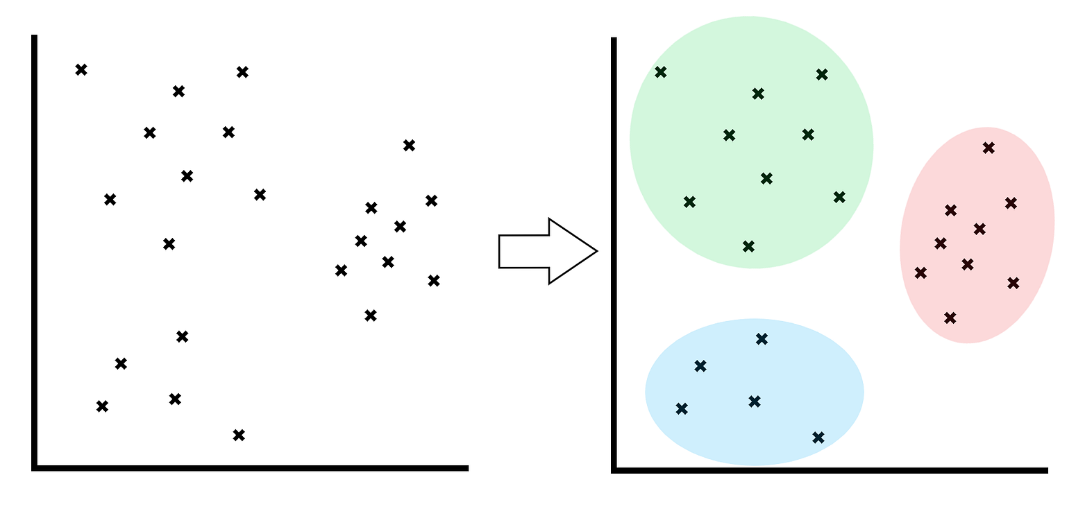
Illustration to show outcome of a clustering algorithm

We’ll be using this clustering algorithm on a dataset made up of image data. Each pixel in an image can be represented by 3 values these correspond to the intensity of each of the colour channels: red, green and blue. Each intensity value will be between 0 and 255.

If we take a pixel value, say, [103, 56, 213] , which is a bright purple colour, we could plot it as a coordinate point on a set of axes (shown below). If we repeat with all of the pixels in an image, we might find that there are ‘clusters’ of points that start to form in the resulting graph. All of the blue pixels will near each other (since they all have similar colour-values), as will all of the green pixels, and the yellow ones. The result may then look something like this:

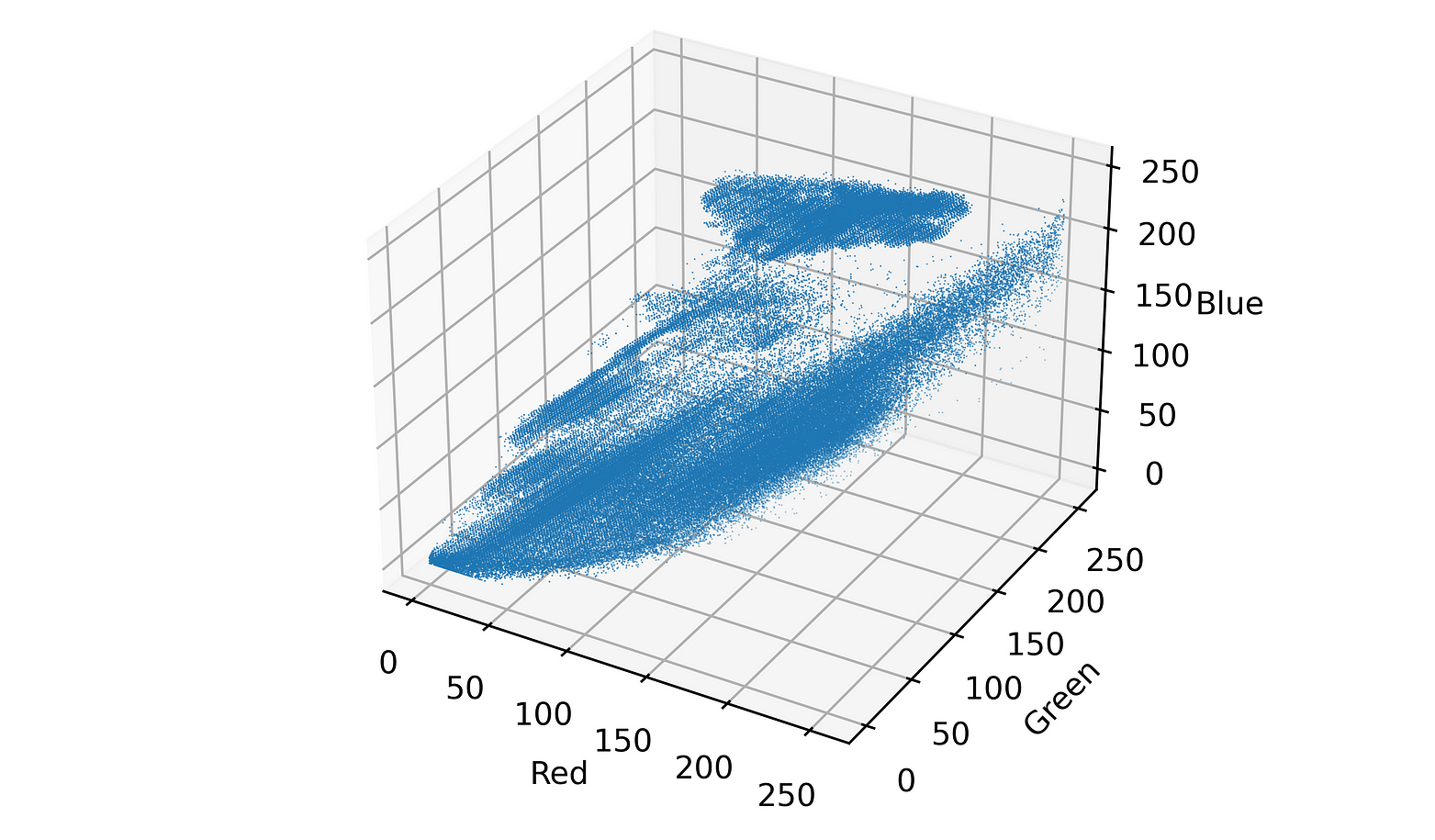
Pixel values plotted in 3D space

While it’s not too easy to see with this fixed perspective, it’s clear that there’s some clusters present in the data where there’s a high density of points close together.

K-Means Clustering

Let’s get into the details of how K-Means clustering works.

We start by choosing a value of k , this will be the number of clusters we want to group our data into. Choosing the right value is an important step, as it can have a big impact on the success of the algorithm. If you happen to know how many different classes your data points fall into, then that is the value you should choose. If not, there are various methods (such as the elbow method) to identify the optimal value of k . The goal is to reduce within-cluster variation (points within a cluster should be close together), and increases between-cluster variation (clusters themselves are as distinct as possible).

For this application, working with images, it’s easy to see how the chosen value impacts the results.

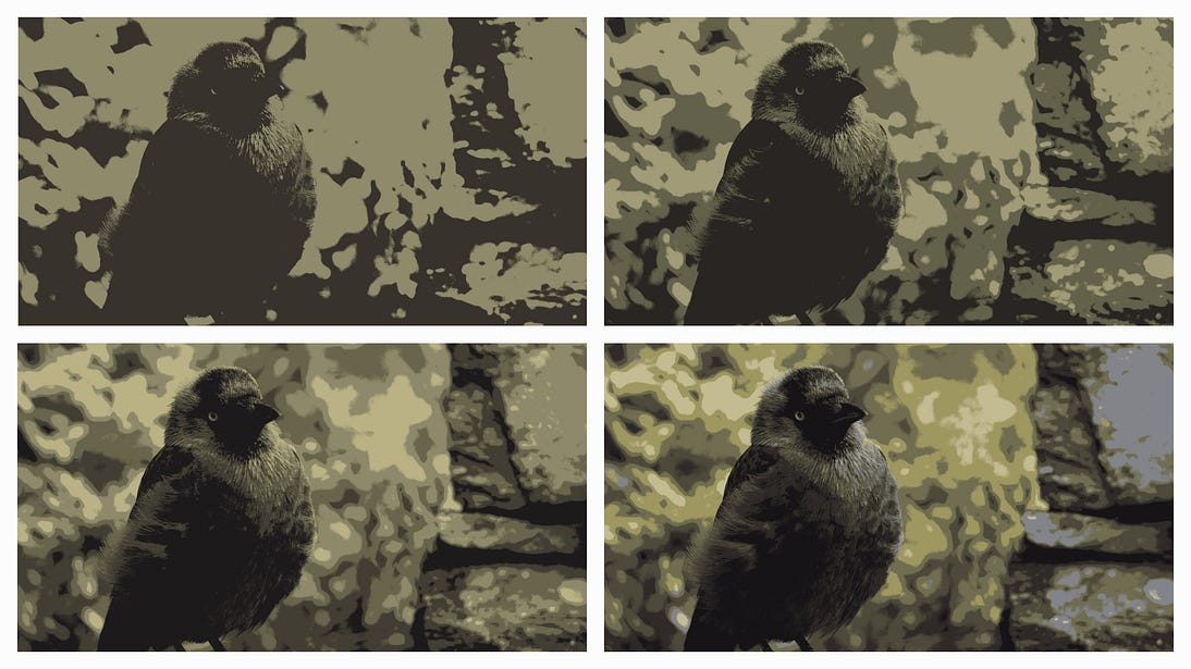
Examples of different values of k: 2, 3, 5, 7 (left to right, top to bottom)

With our value of k chosen, the next step is to set up our initial centroid points these represent the centre of each cluster. We randomly choose a set of coordinates, within the range of possible values, for each of our centroids.

Then the following steps are repeated:

• Work out the distance between every pixel and every centroid
• Assign each pixel to the closest centroid
• For each centroid, find the mean of all allocated pixels, this should be done for each dimension individually.
• ‘move’ the centroids by updating their coordinates to those mean values

This is repeated until the centroids stop moving. This indicates that there are no further changes to the clusters, each pixel is allocated to the nearest cluster, and the centroids are in an optimal position.

Let’s now implement a simple version of this algorithm in Python. This is not a computationally efficient way to perform this process, as we will see during testing, but it is a very straightforward approach.

Later on, we will introduce a more efficient approach using vectorised calculations. This will enable us to work with higher resolution image, dramatically cut down on execution time.

Python Algorithm #1

We’ll start by importing our image and converting it to a pixel array.

img = cv2.imread("bird-small.jpg")

# swap colour channels so that it is displayed correctly
img = cv2.cvtColor(img, cv2.COLOR_BGR2RGB) 

# display image
plt.axis('off')
plt.imshow(img);

# split into channels
r, g, b = cv2.split(img2)

# reformat pixel colours into 1xn array
r = np.array(r.flatten())
g = np.array(g.flatten())
b = np.array(b.flatten())

This image has dimension (267, 400, 3) , that is, height = 267, width = 400, channels = 3. We split the channels into 3 arrays, and then reformatted those to be a 1xn array (a long line of pixel values instead of a pixel grid).

For example, the red channel now looks like this:

[130, 130, 130, …, 145, 156, 159] 

containing 267*400 = 106,800 values

Let’s now define a distance function, which will be used to work out the distance between a pixel and a centroid. For this example, we will use Euclidean distance, given by the following formula:

distance = sqrt( (b0-a0)^2 + (b1-a1)^2 + (b2-a2)^2 ) 

where a and b are the two pixels, and a0, a1, a2, b0, b1, b2 are the colour components of each pixel.

# euclidean distance
def dist(a, b):
    return np.sqrt( (a[0]-b[0])**2 + (a[1]-b[1])**2 + (a[2]-b[2])**2 )

Next we’ll set up the initial centroid positions, and define some parameters for this method.

# number of clusters/centroids
k = 4

# random initial starting points within range 0, 255
centroids = np.array([ [ random.randint(0, 255),
                         random.randint(0, 255),
                         random.randint(0, 255) ] for i in range(k)])

# number of pixels in the image
pixels = len(r)

# exit conditions - stop repeating when max iterations have been reached
# or the centroids stop moving
max_iter = 8
moved = True

Now we can construct the main body of the algorithm.

iter = 0 

while moved and iter <= max_iter:
    iter += 1
    
    # cluster assignments, placeholder array
    assignment = [0]*pixels

    # for each pixel
    for i in range(pixels):

        # compute distance between each pixel and each centroid
        distances = [0]*k
        for j in range(k):
            distances[j] = dist(centroids[j], [r[i], g[i], b[i]] )

         # find minimum distance, returns index (0, .., k-1) of nearest centroid
        nearest = np.argmin(distances)
        
        # will look something like:
        #     [0, 0, 1, 0, 1, 2, 2, 0, ...]
        # with a centroid value assigned to each pixel
        assignment[i] = nearest
        
    prev_centroids= centroids.copy()
    
    # for each cluster, calculate mean of allocated points for each dimension
    for i in range(k):

        # list of array indices of pixels that belong to each cluster
        ind = [j for j in range(pixels) if assignment[j] == i ]

        # check cluster assignment is not empty
        # prevents divide by zero error when calculating mean
        if len(ind) != 0:
            centroids[i][0] = np.mean(r[ind])
            centroids[i][1] = np.mean(g[ind])
            centroids[i][2] = np.mean(b[ind])
        else: 
            centroids[i][0] = 0
            centroids[i][1] = 0
            centroids[i][2] = 0
    
    # check if centroids have moved
    if np.array_equal(centroids, prev_centroids):
        moved = False

With the algorithm complete, we can now reconstruct the image, assigning each pixel the colour of it’s cluster centre to produce the desired effect.

# make copy of colour channels
r_copy = np.array(r.copy())
g_copy = np.array(g.copy())
b_copy = np.array(b.copy())

# update pixels to be the colour of their cluster
for i in range(k):
    ind = [j for j in range(pixels) if assignment[j] == i ]

    r_copy[ind] = centroids[i][0]
    g_copy[ind] = centroids[i][1]
    b_copy[ind] = centroids[i][2]

# compile channels
img2 = np.array([r_copy, g_copy, b_copy])

# transpose to group values into pixels
img2 = img2.transpose()

# reshape list of pixels into height x widgh x channels
img2 = img2.reshape(img.shape)

plt.axis('off')
plt.imshow(img2)

plt.savefig("bird-small(k4).png", format="png", dpi=600)

Testing

As we can see, the image has been reduced to only 4 different colours. However, as expected, this is a very inefficient implementation, taking around 30 seconds to run, and that’s only for a low resolution image.

// k = 4

Initial Random Centroids: [ [ 82 117  80]
                            [134 182 172]
                            [214 107 227]
                            [155  45 225] ]

Final Centroids: [ [ 83  79  62]
                   [130 127  98]
                   [178 171 127]
                   [ 33  31  31] ]

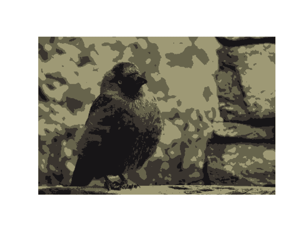
LEFT: Before Clustering, RIGHT: After Clustering (k=4)

Python Algorithm #2 (Optimised with NumPy)

We perform setup similar to before, except we keep the image as a 3d array instead of splitting it into channels. We also rewrite the distance function to work with vectors of values rather than individual points. This allows for more efficient execution as some operations can be done in parallel.

img = import_image("corfu.jpg")

# split image into channels, reformat h x w x c structure 
img = np.array(cv2.split(img))
img = img.transpose(1, 2, 0)

# exit conditions
max_iter = 10
iter = 0
moved = True

# number of clusters
k = 7

# initial cluster centres
clusters = [[random.randint(0, 255) for i in range(3)] for j in range(k) ]

# define distance function
def dist(a, b):
    return (np.sqrt(np.sum( (b-a)**2, 2)))

The main body of the algorithm follows a similar structure, except we use a different encoding method to keep track of which pixels correspond to which cluster, and use 2D masks to index the image, allowing for faster access.

iter = 0
while iter <= max_iter and moved == True:
    iter += 1

    # calculate distance between pixels and cluster, for every cluster
    distances = [dist(img, clusters[i]) for i in range(k)]        

    # index (0, ..., k) of the nearest cluster centre for each pixel
    # produces an array the same shape as the image, instead of pixels,
    # it stores in the index of the nearest cluster
    # this can be used as a mask later on
    nearest = np.argmin(distances, 0) 

    prev_clusters = clusters.copy()
    
    for i in range(k):
        
        # create 1-hot encoded mask of which pixels belong to the cluster
        ind = np.array( np.where(nearest == i, 1, 0), dtype = bool) 

        # apply mask to image to extract subset of pixels 
        subset = img[ind] 

         # calculate mean of the identified subset - update cluster centres
        clusters[i] = [np.round(np.mean(subset[:,0])),
                       np.round(np.mean(subset[:,1])),
                       np.round(np.mean(subset[:,2]))]

        # remove NaN values - replace with 0
        if np.isnan(clusters[i][0]):
            clusters[i][0] = 0
        if np.isnan(clusters[i][1]):
            clusters[i][1] = 0
        if np.isnan(clusters[i][2]):
            clusters[i][2] = 0

    if clusters == prev_clusters:
        moved = False

Now to display the image.

# After the final iteration, the cluster centres represent the pixel colour
# of each cluster. We apply the final version of the array, nearest, as a
# mask to sample colours for each pixel

clusters = np.array(clusters, dtype = int)
img2 = clusters[nearest]

# display image
plt.axis('off')
plt.imshow(img2)

plt.savefig("corfu(k7).png", format="png", dpi=600)

Testing

Testing this version with the image from before, we see a dramatic improvement, with total execution time of less than 1 second. This now allows us to try a larger image, and with a higher max_iter cut-off point (potentially leading to a more accurate result).

The image below has dimensions (2003, 3456) giving it 6,922,368 pixels. This is almost 65 times more than before (106,800 pixels).

With this new implementation, the image takes around 40 seconds to process (for the same value of k). Therefore, processing this same, new image with the previous implementation, would have taken over 15 minutes.

(It’s worth noting that performance is impacted slightly by choice of k due to the structure of the code).

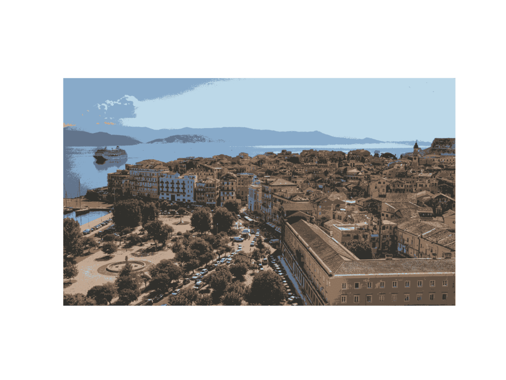
LEFT: Before Clustering, RIGHT: After Clustering (k=7)

Further Optimisations

There are definitely more optimisations that can be made to this code. It could be further vectorised to compute distances for all pixels and all centroids in one go, but it would become a little confusing and difficult to read.

To see even further improvements in performance, we could consider re-writing this algorithm to be able to run on a GPU. As a highly parallel algorithm with many operations that can be performed simultaneously, we could see quite a boost in speed.

Implementing k-means clustering in Python provides a great way to understand the fundamental concept of the algorithm. By exploring an alternate implementation, we have highlighted some optimisations we can make to speed up performance not only in this algorithm, but in many similar procedures too.

References and Reading

• https://www.geeksforgeeks.org/clustering-in-machine-learning/

#MachineLearning #ImageProcessing #Clustering #Algorithms #HandsOnTutorial

Unless otherwise stated, all images are by the author.