Convolution, Kernels & Filters: A Beginner’s Guide to Edge Detection

The Problem of Detecting Edges

I find it interesting how your brain just knows where one object ends and another begins. That instinctive separation is a fundamental part of how we perceive the world. Computers, however? Well, they just need a bit more help.

In computer vision, edge detection is the process of teaching machines to recognise those boundaries, outlines, and transitions in intensity that define structure in an image.

Believe it or not, it’s not as complicated as you might think!

Let’s start with 1 dimension

Let’s start off with just 1 dimension and take a set of random values between 0 and 1:

We can now take a rolling average of this dataset…

• We start with our window on the left hand side of the list of values and take the average of the 3 left-most values.

• We slide our ‘window’ one place to the right and take the average of the next 3 values

• We repeat this process: sliding our window along one place and taking the average of the 3 values it covers, until we reach the right hand side:

Let’s visualise this with a proper data set. Here’s another set of random values between 0 and 1:

We can take a sliding-window average of this dataset, the output of which looks like the following:

The result is a ‘smoothed-out’ version of the original data.

We aren’t limited to just taking a rolling average of 3 elements; we can increase the size of our sliding window to n=5:

Which, when applied to our original dataset, looks like this:

In fact, we can choose any odd number we like, but you’ll notice that the larger the window, the more ‘smoothed’ the output becomes. This is easier to see if we put them side by side. Below, we have n=3 and n=7 sliding window averages applied to the same set of data. The one with the larger window (on the right) looks much less jagged and noisy.

[LEFT] n=3, [RIGHT] n=7

We don’t have to stop here, either! We can take it one step further and look at a weighted sliding-window average.

In the example below, we assign the center element of the window a relative weight of 2, and the 2 elements on the wings, a relative weight of 1. This ensures we retain more of the original shape of the dataset. An operation like this is sometimes called a Gaussian blur – coming from the shape of the Gaussian (Normal) distribution.

To calculate the weighted average, we multiply each element by its weight, add those values together and then divide by the sum of the weights.

Here’s this Gaussian blur applied to our trusty dataset:

This set of values, \begin{bmatrix} 1 & 2 & 1 \end{bmatrix} is known as a kernel, and the sliding-window-weighted-average operation is known as a convolution.

Note. Sometimes we don’t worry about dividing by the sum of the weights at the end. It might mean that all of our output values are 4 times what they should be, but they are still proportional to each other. Depending on our goal, and in use-cases such as edge detection, this step is not important. The other alternative we have is to divide all of the weights by the total sum of the weights. This will perform that final division step implicitly so we don’t have to worry about it. In which case, instead of using \begin{bmatrix} 1 & 2 & 1 \end{bmatrix} as the kernel, we would use \begin{bmatrix} 0.25 & 0.5 & 0.25 \end{bmatrix}.

Convolutions with a different Kernel

What would happen if we took a slightly different kernel, say

\begin{bmatrix} 1 & 0 & -1 \end{bmatrix}

Well let’s take a look at a different, less random, dataset and we’ll see what this kernel can do.

Applying this \( [ \,\, 1 \,\, 0 \,\, -1\,\, ] \) kernel produces the following, somewhat strange-looking output:

It might be easier to see what’s happening here if we overlay the source data and the convolution output over the top of each other:

This convolved data can tell us something interesting about the original dataset:

• Where the value of the convolved data is zero, there’s no change in the height of our source data
• Where the convolved value is close to zero and steady (~0.1) there is a smooth transition in the height of our source data (see the leftmost red bar above)
• Where the convolved value is very high or very low, and jumps suddenly (>0.5, <-0.5) there is a sudden transition in the height of our source data (see the vertical red bars)
• Where the convolved value shows a curve or diagonal (see the right-side red bar) the gradient of the source data is changing – the source data has a curve)

This kernel is finding the gradient of our data source. The height of the output us the ‘steepness’ of the transition.

To then identify the ‘edges’ in our dataset (or areas where there is a sudden transition from one height to another) we can look for values greater than 0.3. or less than -0.3.

Tackling 2 Dimensions

When we move to 2 dimensions, the procedure is largely the same. Since our dataset now has 2 dimensions, our sliding window must as well; it becomes am \( n \times n \) square rather than a \(1\times n\) rectangle.

Performing a convolution is very similar to the 1 dimensional case. We start with the top left data item, and perform the same sliding window operation from before. We slide the window along the rows until we reach the end, move down to the next row, then repeat until we’ve covered each data point.

The biggest difference in 2 dimensions is that we now need a second kernel to find the full gradient of our dataset. Each kernel will find the gradient in one direction: horizontal and vertical. We can then combine these outputs to find the full gradient.

Kernel to find the gradient in the horizontal direction: \begin{bmatrix} -1 & 0 & +1 \\ -2 & 0 & +2 \\ -1 & 0 & +1 \end{bmatrix}

Kernel to find the gradient in the vertical direction: \begin{bmatrix} +1 & +2 &+1 \\ 0 & 0 & 0 \\ -1 & -2 & -1 \end{bmatrix}

These Kernels are known as the Sobel filters.

After we’ve done this for every element of our source data, we can scale the values of the output to make sure they’re all still within that 0-1 range.

To find the gradient of the data in 2 dimensions, we first find the horizontal gradient by performing a convolution with the horizontal Sobel filter e.g. :

You’ll sometimes see this \(\otimes\) symbol used to mean: ‘multiply each corresponding element and add them together’.

Then we find the vertical gradient, by performing a convolution with the vertical Sobel filter, e.g. :

And then combine them as follows:

\[ grad, \Delta = \sqrt{ {grad_x}^2 + {grad_y}^2} = \sqrt{ {0.32}^2 + {1.16}^2} =1.2033\dots \]

Where \( grad_x , and grad_y \) are the outputs from the two convolution steps above. We then repeat this for every element of the source data.

Let’s now see some examples with actual images.

A quick aside

Each pixel in an image is made up of 3 values: one for red, one for green and one for blue. These values are usually between 0 and 255, but we can scale them such that they are between 0 and 1.

For example, \( [ 66, 245, 224] \rightarrow [ 0.2588, 0.9608, 0.8784] \) results in this nice teal color.

So far, all of our convolution examples have used a single value per cell. Therefore, we must combine the 3 colour channel values into a single number.

To do this, we convert our image to black and white. This gives us a single value per pixel – the lightness or value of the pixel. 0 is pure black, 1 is pure white. But don’t worry, we will still be able to identify the edges in the image.

Let’s see some examples

Firstly, to see why we need 2 kernels to find the gradient in 2 dimensions, let’s see what happens if we use just one of them. We’ll start with this image and apply only the horizontal version and only the vertical version of the Sobel filter:

[left to right] Original image, horizontal Sobel Filter applied, vertical Sobel filter applied.

Applying the horizontal Sobel filter allows us to identify where there are sudden changes in lightness values moving from left to right – this gives us the vertical edges in the image. Similarly, the vertical filter, identifies changes in lightness from top to bottom which gives us the horizontal edges.

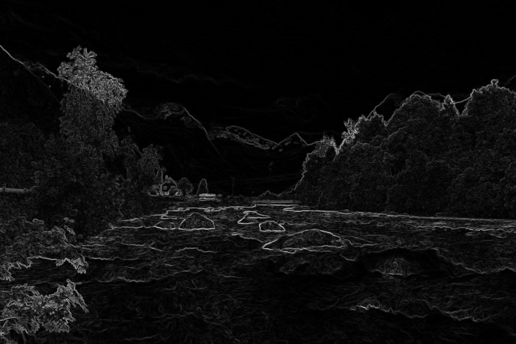
Now, if we combine these using the formula we saw earlier, we get something that looks like this:

And for clarity, we’ll overlay this on top of the (black and white version of the) original image:

Changing Channel

Depending on the image you’re using, there might be a better way to find edges than using black and white. Let’s mix things up with a different example:

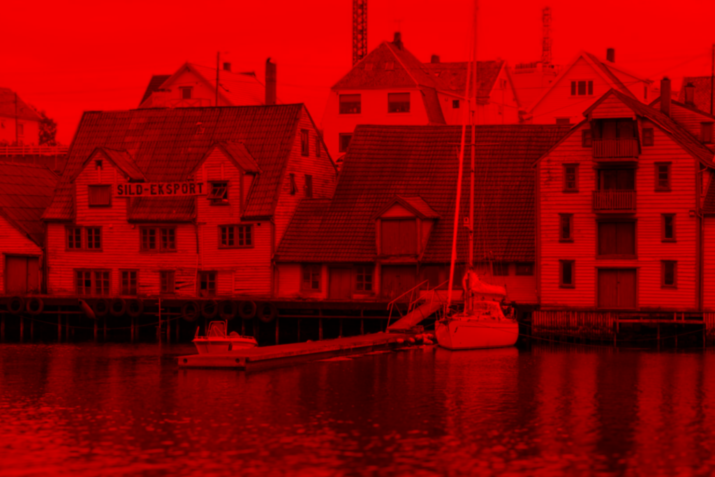
If we look at each of the three color channels in this image, we find more contrast in the red and the green, and far less in the blue channel.

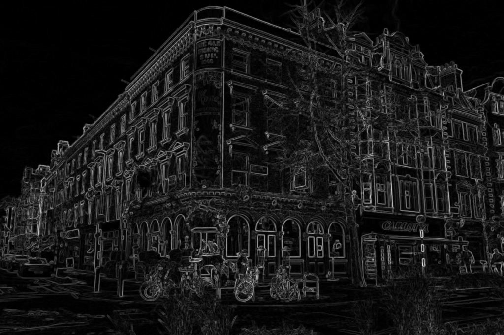
If we apply our edge detection procedure again to each of these channels, we get some slight variation in the results.

Now don’t get me wrong, these are all pretty similar. I’m not trying to suggest that one is miles better than the other – they all get the overall shape correct.

However, since there is less contrast in the blue channel, the algorithm has a harder time picking out the fine details, particularly in the buildings.

But if you take a second, zoom in, give it a really close look, then you might start to notice some of the more subtle differences between the other three.

Ultimately, using a greyscale image will probably give you the best all-round result the majority of the time. However, depending on your use case, we can sometimes get better details and clarity by using a different colour channel.

The secret trick I’ve snuck past you so far

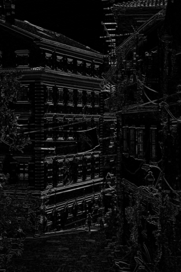
Take a look at these two edge detections. Do you notice any differences between them?

The first output has far more detail and clarity than the second. We don’t live in a perfect world with perfectly sharp images in perfect lighting. Sometimes our images will be low quality and be quite noisy like this:

In cases like these, we first apply a blur to our image to reduce the impact of the random variations within the image.

It takes our noisy image and reduces it to something much smoother, albeit with slightly less detail.

It’s a little difficult to see, but the edges are just slightly softer and the noise is a little less prominent. look at the trim along the hut, the detail of the flag, and the colour noise in the clouds. It only needs to be subtle, just enough to blend in the random variation with the pixels around it. If we blur the image too much, we’ll start to lose important details and the quality of our output will diminish.

To perform a Gaussian blur, we convolve our image using the following kernel. You may notice it’s similar to the 1D version we saw earlier.

\[ \frac{1}{16} \begin{bmatrix} 1 & 2 & 1 \\ 2 & 4 & 2 \\ 1 & 2 & 1 \end{bmatrix} \]

Python implementation

Want to try this out for yourself? Try out the python code below! You may need to install some packages to get it working – check the imports at the top of the script.

import cv2
import numpy as np
import matplotlib.pyplot as plt
from scipy.signal import convolve2d

# === Config ===
image_path = 'filename.jpg'            # Image filename
apply_blur = True               # Optional blur
sobel_direction = 'both'       # Options: 'horizontal', 'vertical', or 'both'
channel_mode = 'gray'           # Options: 'gray', 'red', 'green', 'blue'
threshold_value = 140           # Edge threshold for overlay (0–255)

# === Outputs ===
original = False         # Output pre-processed image 
Sobel = True             # Output of sobel filter
overlay_edges = False    # Overlay red edges on pre-processed image
overlay_over = 'color'   # Overlay edges on top of 'color' or 'gray' image
 

# Load image
image_bgr = cv2.imread(image_path)
if image_bgr is None:
    raise FileNotFoundError(f"Could not load image: {image_path}")

# === Convert to working input based on selected channel ===
if channel_mode == 'gray':
    input_image = cv2.cvtColor(image_bgr, cv2.COLOR_BGR2GRAY)
elif channel_mode == 'red':
    input_image = image_bgr[:, :, 2]  # OpenCV uses BGR
elif channel_mode == 'green':
    input_image = image_bgr[:, :, 1]
elif channel_mode == 'blue':
    input_image = image_bgr[:, :, 0]
else:
    raise ValueError("channel_mode must be 'gray', 'red', 'green', or 'blue'")

# === Optional blur ===
if apply_blur:
    input_image = cv2.GaussianBlur(input_image, (5, 5), sigmaX=1.0)

# === Prepare for convolution ===
image_float = input_image.astype(np.float32) / 255.0

# === Define Sobel kernels ===
sobel_horizontal = np.array([
    [-1, 0, 1],
    [-2, 0, 2],
    [-1, 0, 1]
], dtype=np.float32)

sobel_vertical = np.array([
    [-1, -2, -1],
    [ 0,  0,  0],
    [ 1,  2,  1]
], dtype=np.float32)

# === Apply convolution based on direction ===
if sobel_direction == 'horizontal':
    convolved = convolve2d(image_float, sobel_horizontal, mode='same', boundary='symm')
elif sobel_direction == 'vertical':
    convolved = convolve2d(image_float, sobel_vertical, mode='same', boundary='symm')
elif sobel_direction == 'both':
    sobel_x = convolve2d(image_float, sobel_horizontal, mode='same', boundary='symm')
    sobel_y = convolve2d(image_float, sobel_vertical, mode='same', boundary='symm')
    convolved = np.sqrt(sobel_x**2 + sobel_y**2)  # gradient magnitude
else:
    raise ValueError("sobel_direction must be 'horizontal', 'vertical', or 'both'")

# === Normalize convolved result ===
if sobel_direction in ['horizontal', 'vertical']:
    convolved_norm = np.abs(convolved)
    convolved_norm = (convolved_norm - convolved_norm.min()) / (convolved_norm.max() - convolved_norm.min())
else:
    # already magnitude, just normalize
    convolved_norm = (convolved - convolved.min()) / (convolved.max() - convolved.min())

edge_strength = (convolved_norm * 255).astype(np.uint8)

# === Create overlay image ===
if overlay_edges:
    # Threshold to isolate strong edges
    _, binary_mask = cv2.threshold(edge_strength, threshold_value, 255, cv2.THRESH_BINARY)

    if overlay_over == 'color':
        base_rgb = cv2.cvtColor(image_bgr, cv2.COLOR_BGR2RGB)
    elif overlay_over == 'gray':
        base_rgb = cv2.cvtColor(input_image, cv2.COLOR_BGR2RGB)
    else:
        raise ValueError("overlay_over must be 'gray' or 'color'")


    # Red-only edge layer
    edge_overlay = np.zeros_like(base_rgb)
    edge_overlay[:, :, 0] = binary_mask

    # Blend
    overlay = cv2.addWeighted(base_rgb, 1.0, edge_overlay, 0.7, 0)
else:
    overlay = None


# === Plotting ===
num_plots = 0
if original:
    num_plots += 1
if Sobel:
    num_plots += 1
if overlay_edges:
    num_plots += 1
plot_idx = 1
plt.figure(figsize=(5 * num_plots, 5))


# Original
if original:
    plt.subplot(1, num_plots, plot_idx)
    plt.axis('off')
    if channel_mode == 'gray':
        plt.imshow(input_image, cmap='gray')
    else:
        # Create empty RGB image and set the selected channel
        channel_rgb = np.zeros((*input_image.shape, 3), dtype=np.uint8)
        channel_index = {'blue': 2, 'green': 1, 'red': 0}[channel_mode]
        channel_rgb[:, :, channel_index] = input_image
        plt.imshow(channel_rgb)
    plot_idx += 1

# Sobel result
if Sobel:
    plt.subplot(1, num_plots, plot_idx)
    plt.axis('off')
    plt.imshow(convolved_norm, cmap='gray')
    plot_idx += 1

# Overlay
if overlay is not None:
    plt.subplot(1, num_plots, plot_idx)
    plt.axis('off')
    plt.imshow(overlay)
    plot_idx += 1

plt.tight_layout()
plt.show()

Wrapping up

Edge detection might seem like a simple idea but as we’ve seen, it rests on some rather simple and creative math. Convolutions slide filters across pixels, kernels act as little pattern detectors, and gradients give us a way to measure change. Together, they help computers spot the outlines that shape everything from cats to cars to street signs.

Edge detection is one of the foundations of image processing and computer vision. Whether you’re moving on to object recognition, segmentation, or neural networks, these concepts will keep showing up.

Enjoyed this read? Check out this article on image segmentation – another image processing technique:

I’ll leave you with a couple more examples to take a look at for some more inspiration.

If you made it this far, thank you!